I trained a neural network in Google Sheets

Some of the most ingenious ideas come from taking something that exists in one medium, and constraining it into another---like reproducing an expensive dish on a tight budget or walking around a city without a map. The same principle applies here: I’m taking something that exists on the frontier of data science---neural networks---and recreating it in an environment one step above doing math by hand. Along the way, I’m forced to find creative workarounds to problems I didn’t see coming, all the while strengthening my understanding of (and hopefully yours too) both Sheets and machine learning.

70,000 images, 614,656 pixels, and 29 years

The model is fit on the MNIST dataset, consisting of 70,000 grayscale 28\(\times\)28 images of hand-written digits (0 through 9), each with a corresponding label, which my model tries to predict.

Training a classifier on this dataset is nothing new---MNIST is a staple in the world of computer vision, and has been around since 1998. What’s not new is the implementation.

Googling “training a neural network in Google Sheets” gets you a few results that appear to do something similar to what I’m doing, but differ in two key ways. One, I’m not importing the model from another source (like PyTorch or TensorFlow), using any code within Sheets (like Google Apps Script), or Add-Ons (like OpenSolver). Solutions that “train” neural networks in Sheets usually end up using one of these shortcuts, which solve some of the fundamental problems with trying to train a model in Sheets, but take away from the point of creating the network in Sheets in the first place.

Of the remaining online solutions that don’t rely on third-party applications, most of them train models that are extremely simple, with relatively few neurons or training iterations, and solve problems that are fairly basic. While it’s true that these solutions do indeed train a model entirely in Sheets, they fail to push the frontier of what’s possible within Sheets.

My model is different: it’s a fully-connected multi-layer perceptron (MLP), that has 784 input neurons (one for each of the pixel values in the 28\(\times\)28 MNIST image), followed by a 128 neuron hidden layer, a ReLU activation function, and finally 10 output nodes, one for each digit, that represent how likely the input is a particular label. In an abbreviated form, this model is a 784-128-10 MLP.

One step forward, one step back

As a high-level overview of what this model does, each hidden layer node (128 total), “learns” 784 weight values, one for each of the 784 input nodes, or each grayscale pixel value in the original image. Each of those 784 weights are multiplied by their corresponding pixel and added together before a “learned” bias term is added to the sum. If it makes it easier to see in linear algebra terms, this can be represented by the formula \(XW_1 + b_1\), where X is a singular input image matrix (size 1\(\times\)784), \(W_1\) is the weight matrix (size 784\(\times\)128), and \(b_1\) are the bias terms (one for each of the 128 hidden layer neurons).

Before continuing the process in the next layer, however, the ReLU activation function takes each of the 128 sums (or equivalently, the \(XW_1 + b_1\) result) and replaces all the negative sums with 0, leaving the positive sums as is. The main purpose of this function is to allow the network to learn non-linear, complex patterns, since the ReLU is itself non-linear.

The final output layer (10 nodes) repeats this operation, but without the ReLU activation function at the end. That is, each of the 10 nodes “learns” 128 weight values, one for each of the 128 hidden layer outputs, and multiplies those weight values pairwise with the corresponding hidden layer results, before adding in a “learned” bias term. This entire process can be summarized with the formula \(\text{ReLU}(XW_1 + b_1)W_2 + b_2\), the result of which represents the 10 outputs (one for each digit) of the model, called the logits. To turn those logits into probabilities, I use a softmax function.

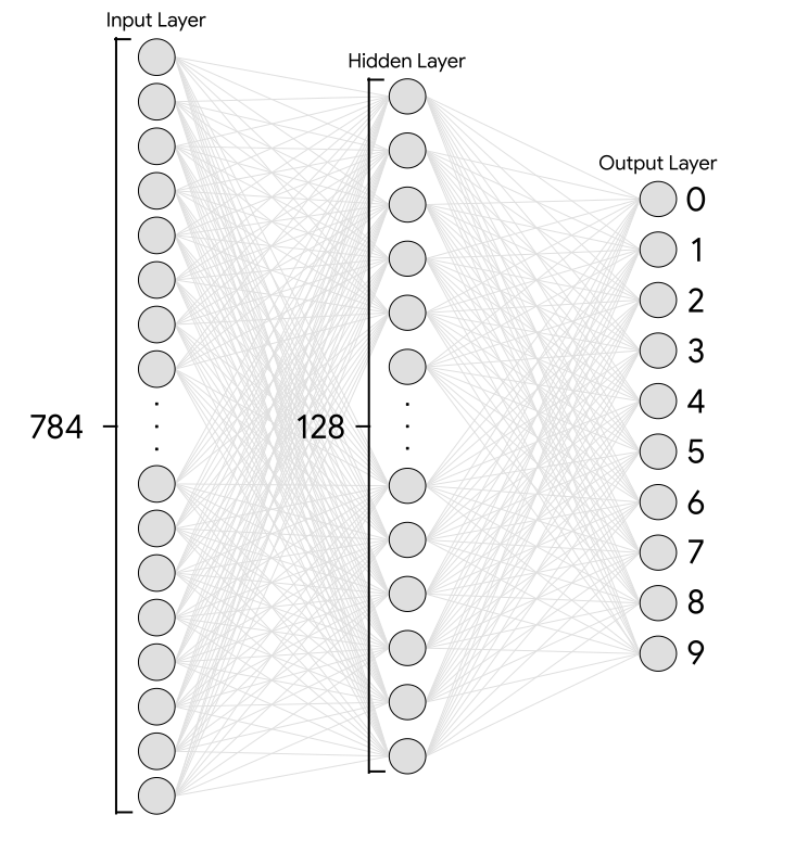
A visualization of the model, where each connection represents a multiplication of a weight and input value.

Up to this point, these calculations are what’s known as a “forward pass,” which just calculates the result of the model. A forward pass can perform the task of classification by taking in an image and giving a probability of each digit, but that probability distribution isn’t necessarily good. For the model to “learn,” it needs to train each of the “learnable” weight values (of which there are \(784\times 128+128+128 \times 10+10 = 101{\small,}770\)) to use in the forward pass calculation.

This “learning” is called backpropagation, and involves quantifying how wrong the forward pass was, then changing all of the weights, or parameters, to make the model not as wrong. The quantification is done via a loss function---in this case cross-entropy loss---and the changing of weights is done by taking the derivative of the loss function with respect to each parameter. The derivative shows how adjusting each parameter would change the loss, so to update weights, I just “step” each parameter in the direction that appears to lower the loss (or the “wrongness”).

While the math behind the network isn’t too important for understanding the purpose of this project, it helps you appreciate the number of computations that underlie such a classifier.

After writing out the math for the forward pass, and deriving the steps required for backpropagation, I can then translate that math into Python code, utilizing the NumPy package for each of the calculations.

train_size = 4000
X = train_data.data[:train_size].numpy()/255 # make values range from [0,1]
y = train_data.targets[:train_size].numpy()
k = 10 # number of classes
d = 784 # dimensionality of the input
h = 128 # size of hidden layer
step_size = 0.1 # proportional to learning rate

w = np.genfromtxt('weights.csv') # same as sheets
b1 = w[128*784:128*784+128] # layer 1 biases
b2 = w[-10:] # layer 2 biases 
W1 = w[:128*784].reshape(h,d).T # layer 1 weights
W2 = w[128*784+128:-10].reshape(k,h).T # layer 2 weights

epochs = 7
for t in range(epochs):
    n = len(X) # number of points
    X_epoch = X.reshape(n, -1) # (n, 1, 28, 28) => (n, 784)
    hL = np.maximum(0, X_epoch @ W1 + b1) # (n, d) @ (d, h): (n, h)
    logits = hL @ W2 + b2 # (n, h) @ (h, k): (n, k)

    probs = np.exp(logits) # (n, k)
    probs /= probs.sum(1, keepdims=True) # (n, k)

    neg_log_probs = -np.log(probs[range(n),y]) # (n,)
    loss = neg_log_probs.sum() / n # (1)
    
    dlogits = probs # (n, k)
    dlogits[range(n),y] -= 1 # (n, k)

    db2 = dlogits.sum(0) # (n, k) => (k)
    dW2 = hL.T @ dlogits # (n, h).T @ (n, k): (h, k) 

    dhL = dlogits @ W2.T # (n, k) @ (h, k).T: (n, h) 
    dhL[hL <= 0] = 0 # (n, h)
    dW1 = X_epoch.T @ dhL # (n, d).T @ (n, h): (d, h)
    db1 = dhL.sum(0) # (n, h) => (h)

    W1  -= step_size * dW1 / n # (d, h)
    b1  -= step_size * db1 / n # (h)
    W2 -= step_size * dW2 / n # (h, k)
    b2 -= step_size * db2 / n # (k)
    
    train_preds = model(b1, W1, b2, W2, X_epoch.reshape(n, 784)).argmax(1)
    train_acc = (train_preds == y).sum() / n
    print('Epoch:', t+1,'Train Accuracy:', train_acc, 'Train Loss:', loss)

From here, all that’s left to do is convert each line of NumPy into cells in Sheets.

A single calculation in Sheets

The first major hurdle comes from storing the data. MNIST contains 70,000 images, each of which correspond to 784 pixels and 1 label. That means storing 70 thousand images in a Spreadsheet requires a minimum of \(70{\small,}000 \times (784+1) = 54{\small,}950{\small,}000\) cells (since each pixel and label would require their own cell) far above the 10,000,000 cell limit for Sheets files. In order to fit this restriction, I cut the dataset size down to 5,000 images, which was further split into 4,000 training points, 500 validation points to artificially test my model, and 500 test points as the final evaluation set. This brought the cell count for storing the data to \(5{\small,}000 \times 785 = 3{\small,}925{\small,}000\) cells, leaving around 6 million for training and testing.

In a similar vein, I need to initialize each of the 101,770 total parameter values, store them, then update them for each pass through the data. Since training occurs in a loop, with weights being updated in each iteration based on their previous values, I have to store each of the weight values for every loop iteration. To accommodate this, I place each of the parameters for a given training iteration in a single column with over 100,000 rows, and the next iteration’s weights in the column to the right.

Finally, to ensure calculation is even possible, I need to restrict the amount of data that can pass through the network at one time. While it would be ideal to use all the data at once to update weights (allowing me to increase the number of times the model sees the training data), doing so for 4,000 training points hits Sheets’ calculation limit, so I’m constrained to passing 500 data points through the network at once (called a batch). That amounts to 8 batches per epoch, where an epoch is a full pass through the entire training set.

With the training structure in shape, I need to translate individual NumPy lines to Google Sheets functions. While lines involving scalar variables can be easily constructed by just putting the same number in a single cell, lines that perform calculations prove considerably more difficult. Take the following line that computes the output of the hidden layer in a forward pass of the data, for instance:

Here, X_batch represents the input images within the current batch. In the Sheets formula for the first batch of the first epoch, X_batch translates to:

Let’s work backwards to understand why. First, the batch indices are given in cell C5, in the format “1,500,” meaning the subset of training points to use for this batch begins at index 1 and ends at index 500. INDEX(SPLIT(C$5,","),1,1) splits the contents of this cell by the delimiter "," and then takes the value of the result at column 1, row 1, which corresponds to “1” in this case. Note that the $ just makes the cell reference to C5 always stay at row number 5, while the column reference might change to D, for instance, if the same formula were copied over to the column to the right. The same logic applies for the almost-duplicate second use case of the INDEX and SPLIT formula, which obtains “500” from C5.

Then, the result "X_train!$A$"&INDEX(SPLIT(C$5,","),1,1)&":$ADD$"&INDEX(SPLIT(C$5,","),1,2) forms the string "X_train!A$1:ADD$500" since & symbolizes concatenation. INDIRECT ties everything together by making the string actually reference the appropriate input data for the given batch indices, making it truly the same as the variable X_batch.

Multiplying X_batch with W1, the weight matrix of the hidden layer, yields the following Sheets formula:

Or, if I replace part of the Sheets formula with X_batch for clarity:

Again starting from the inside, WRAPCOLS(B12:B100363,784) takes the weights for the hidden layer (which are all in one column) and translates them into a matrix that has 784 values for each column (or equivalently, 784 rows). MMULT is fairly self explanatory---it multiplies X_batch with WRAPCOLS(B12:B100363,784), which is the same as X_batch @ W1 in code.

Adding b1 to the X_batch @ W1 result is equivalent to:

Where TRANSPOSE(B100364:B100491) transforms the biases so that they can be added to the previous multiplication result, via an ARRAYFORMULA that maps the addition across the two matrices.

Finally, the ReLU functionality, represented in code by np.maximum(0, X_batch @ W1 + b1) can be accomplished in Sheets with:

Which MAPs a LAMBDA function, or a function applied to each value in the given matrix. This LAMBDA is the aforementioned ReLU, which just takes the “cell” and returns the MAX value between the “cell” itself and 0. After evaluating this part of the function, the Sheets result is equivalent to hL, the hidden layer.

All of that represents a single, fairly simple line of code in NumPy, translated entirely to Sheets:

The 98.99% compression algorithm

As you can imagine, debugging is particularly frustrating. Since whitespace and parameter names are not permitted in Sheets formulas, I’m forced to interpret multiple lines of concise NumPy code as one giant string of formulas. Plus, since later NumPy lines use previously calculated values, I have to keep building from the same Sheets formulas as I progress through translating the code, rather than starting new each time.

There’s one helpful trick to ease in interpretability, however. I could store these intermediate values (like logits, for example) in cells within the Sheet, then reference those cells whenever I need to make a calculation involving logits. The only issue with this approach is the intermediate results are typically too large to store: the logits matrix is of size \(500\times 10\), meaning I’d have to store 5,000 values. While not too large of a quantity for a single backpropagation step, I’d need to store this for every batch, which quickly pushes the file to the 10 million cell restriction.

To limit the amount of space storing intermediate values takes up, I could instead push each of those 5,000 numbers into a single cell by flattening the matrix and concatenating all of the values together, separated by commas, to form a 5,000 long comma-separated list. Since I know the dimensions of the original matrix, I can perfectly reconstruct it from the concatenated result, by simply “unflattening” the list. The one caveat to this workaround is a 50,000 character limit on strings within a cell in Sheets, meaning every value in the list must be associated with about 9 characters. Rounding the logits to 5 digits does just that---since most of the logits are between -1 and 1, there’s one character for the one’s place, one for the decimal, five for the fractional part, one for the comma, and potentially one for a negative sign, yielding about 9 characters for each of the 5,000 numbers.

Rounding loses some information---I can no longer reconstruct the original matrix beyond the fifth decimal point for each value---but from testing, the fifth decimal is enough for accurate results almost exactly equivalent to their NumPy counterparts.

The above flattening and rounding for logits takes place in cell C9 in the train Sheet, and looks like this:

To reconstruct the logits matrix, I can just use this Sheets formula:

Which constructs a matrix from the C9 cell by first splitting the contents of the cell by the character they were joined with (","), then using that 5,000 length list to make a matrix with 10 values per row (and 500 per column), almost exactly equivalent to the original logits.

With the trick of storing intermediate values in hand, there’s some ease in translating the rest of the NumPy lines. For the most part, they are all matrix operations, and built up from a subset of Sheets formulas. Completing a singular batch of training, or translating each of the training loop lines of NumPy, amounts to 244 total Sheets function calls but only 29 unique Sheets function uses:

Most of the functions are self explanatory, since almost all of them deal with transforming matrices in some way. Interestingly, non-matrix operations SPLIT and INDEX are the most frequent, since they are used in tandem to obtain the index bounds for each batch, which is necessary for referencing the appropriate images and labels, as well as measuring the batch length. SPLIT slightly edges out INDEX for most use, since it contains an additional use case in splitting a comma-separated list to reconstruct intermediate matrix values.

The benefit of having relatively few functions used, at least compared to the total function calls, is that each calculation is fairly simple to interpret, as it’s built off the same few steps (just repeated several times).

Training to the limit

After filling in cells for a single batch of training, continuing to train for further iterations is simply a matter of copy-pasting formulas into an adjacent column. Since the training structure is set up to maintain references to certain cells by relative positioning, properly written formulas needn’t be changed as training pushes forward, saving a lot of manual effort.

The key metric to look at to ensure correctness in implementation is the training loss (loss), which should generally decrease batch-to-batch---after all, minimizing the training loss is the entire objective of the neural network’s training process. Complementary to the decrease in training loss is the increase in training accuracy, and more importantly, the validation set’s accuracy. Since the validation set isn’t used at all in training, it’s a good estimate of how the model might work on unseen data. Again, while not necessarily true of each batch, seeing both of these metrics trend in their desired directions indicates my formulas are doing what they are supposed to.

Note that there’s a significant lag when adding each additional training batch, as millions of calculations need to occur for a training loop to end. In order to prevent crashes, I only add a few batches at a time, which typically take less than a minute to fully calculate, then add more when they are completely done.

The 10,000,000 cell limit also comes back into play here. Since each of the batch columns contains over 100,000 rows and I’m already using nearly 4 million cells to store the data, I can only run 7 full epochs (8 batches per epoch, so 7 full epochs means \(8\times 7\times 101{\small,}770 = 5{\small,}699{\small,}120\) cells) before running out of computing space. After pushing the Spreadsheet to its limit, I’m left with a train accuracy of 75.4% and a validation accuracy of 73.8%.

Though some ways away from state-of-the-art (some models achieve a less than 1% error rate), and while more epochs would certainly help increase accuracy, the result is more than 60 percentage points above what would be expected from randomly guessing (10% accuracy), so the model is certainly noteworthy.

The last stage in the lifecycle of this Sheets model is to deploy it on an unseen test set. To do so simply requires adjusting the previously used accuracy calculations to be compatible with the testing data, by swapping out the cell references to the training and validation datasets. Upon completing the adjustment, my model earns a test set accuracy similar to that of training and validation: 72.4%, meaning the model is fundamentally understanding patterns about hand-written digits, since it generalizes well to this new data rather than simply regurgitating patterns exclusive to the training set.

While 72.4% accuracy explains how well the model predicts digits, it doesn’t explain what types of predictions the model actually makes, nor how the 27.6% error rate comes about. I can answer those questions via an aptly named confusion matrix, which visualizes the model’s predictions against the true values in a 2D table. There isn’t Python code to explicitly reference for this visual, but each of the values in the below output is based on a modified version of the test accuracy calculation. Specifically, I filter the test set to only include digits that match a particular label, then count how many times the model predicts each of the 10 digits for that particular label (repeating this for all 10 numbers):

Reading the chart is simple. For instance, take the pred_label value 3 and the true_label value 8. Since the corresponding value for those coordinates is 2, this means that there are 2 occurrences of when the model predicted a digit was a 3, when it was really an 8. Conditional formatting shading the diagonal indicates that the model is correct most of the time---it’s predicted digit matches the true digit. However, the chart makes it clear that the model struggles the most with the digit 5, as indicated by the spread of predicted values in its row. Only 2 predictions of 5 are correct (which happen to be the only 2 predictions of 5), and the model often confuses 5s with 3s and 0s. There’s also some confusion with 4s and 9s, as well as 7s and 9s.

To understand why these errors might be happening, I can set up a visualizer for the image inputs to see both the types of images the model gets right, and the types it gets wrong. Since visualizing all 500 inputs would force the Spreadsheet beyond the 10 million cell limit, I can instead set up a cell to specify a single test index, then utilize INDIRECT to reference that cell and obtain the corresponding image, label, and model prediction.

Test index 30 allows for some insight into the errors:

This image is labeled as a 5, but could plausibly be a 0, with the bottom half of the image resembling a full circle.

The same applies for test index 101, which is truly a 5, but predicted a 3:

There’s some semblance of the shape of a 3, which is enough to push the model to make the incorrect classification. Hence, although the 27.6% error rate is relatively high in comparison to what more complex models are able to achieve, paradoxically, several of the errors that the model makes are somewhat acceptable, given that they stem from understandable digit shape misreadings.

A Google Sheet is a metaphor

The final tab in the Spreadsheet is meta, which contains information about the cell counts in each of the Sheets within the file, and their sum. In total, there are 9,829,555 cells used in the initialization, training, and testing of the neural network, with the most cells being allocated to the training Sheets, both for storing the training data (3,136,000 cells) and actually running the training loops (5,903,298 cells).

Poetically, this meta tab serves as an apt meta-commentary on the process of developing a neural network entirely in Sheets. The tab was created solely to track how close I was getting to the 10 million cell limit as I built the model, which was by far the most challenging aspect of completing this project, since it placed a hard limit on its scope: restricting the dataset size, model complexity, and number training iterations. It’s a similar story for each training pass, which had to be reduced to 500 points per iteration to mitigate high computation cost, thereby pushing the training process to the 10 million cell limit, faster. Without these limits, the model could have seen the entire MNIST database, added additional hidden layers, or, if nothing else, continued to train in its current state.

But the pain of dealing with those restrictions was countered by the joy of finding clever workarounds. Figuring out how to safely store thousands of values into a single cell to aid in debugging was incredibly exciting, only because it solved a problem that wouldn’t have existed if not for this project.

The same goes for translating NumPy functions over to Sheets. While the process itself was tedious, understanding how to represent something like boolean indexing in NumPy (filtering a matrix by a condition, then performing an operation on that filtered subset) allowed me to think about matrices in a different way---again, a way that existed only because I made it exist.

Above all else, successfully representing an accurate and in-depth neural network in a software as basic as vanilla Google Sheets, with only 29 different functions in the training process, illustrates that even the most seemingly complex computer science phenomena can be distilled to basics---and successfully understood by anyone.